STATISTICAL PHYSICS
PAPER A1, SECOND YEAR
| |
 |
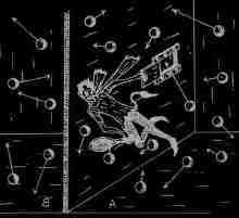
(drawing by G. Gamow) |
Prof Alexander Schekochihin and Prof Andrew Boothroyd
NOTE: The course this year will largely follow the pattern of 2013-14, for which all the materials (including lecture notes) are available here. We give all the essential links below, with updates where applicable. A pre-historic version of the course, 2011-12, is here (but the order of presentation, the notes and the problem sets were different then).
What you see below will initially be lecture content, notes and downloads from the 2013-14 course.
Where appropriate, these will be updated and marked as such (in RED!).
So do please visit this website regularly if you wish to stay abreast of the latest developments.
LECTURE NOTES: This year, I intend to produce a LaTeX'ed version of my Lecture Notes (the hand-written ones linked below).
The current version (20.02.2015) of the pdf file containing this write-up is linked here.
This file will accrete sections as we proceed.
I will be very grateful for your feedback: comments, error corrections, views etc.
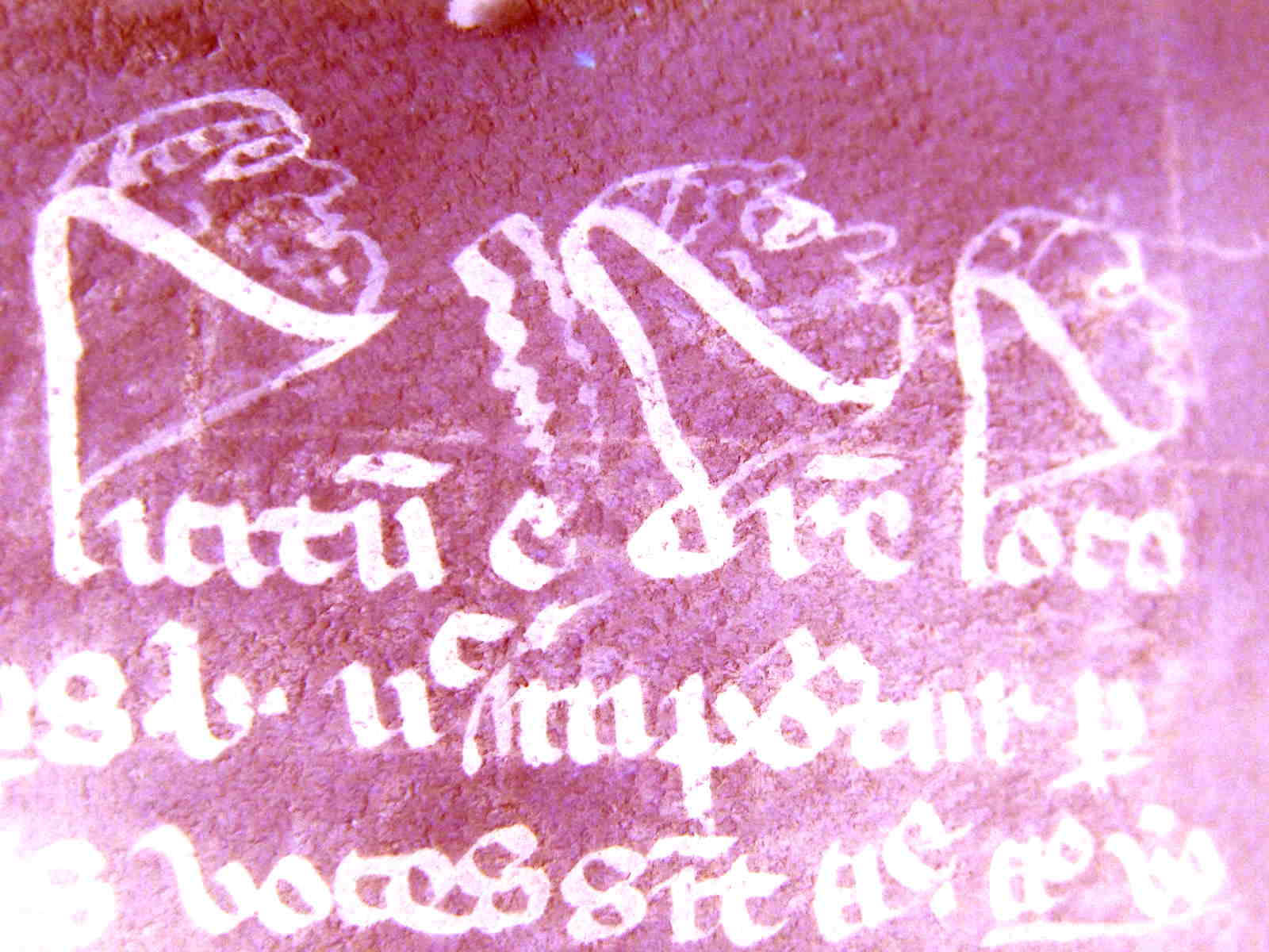
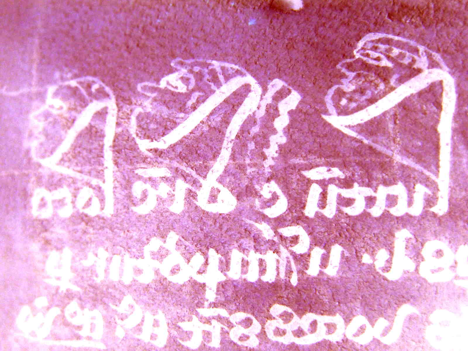
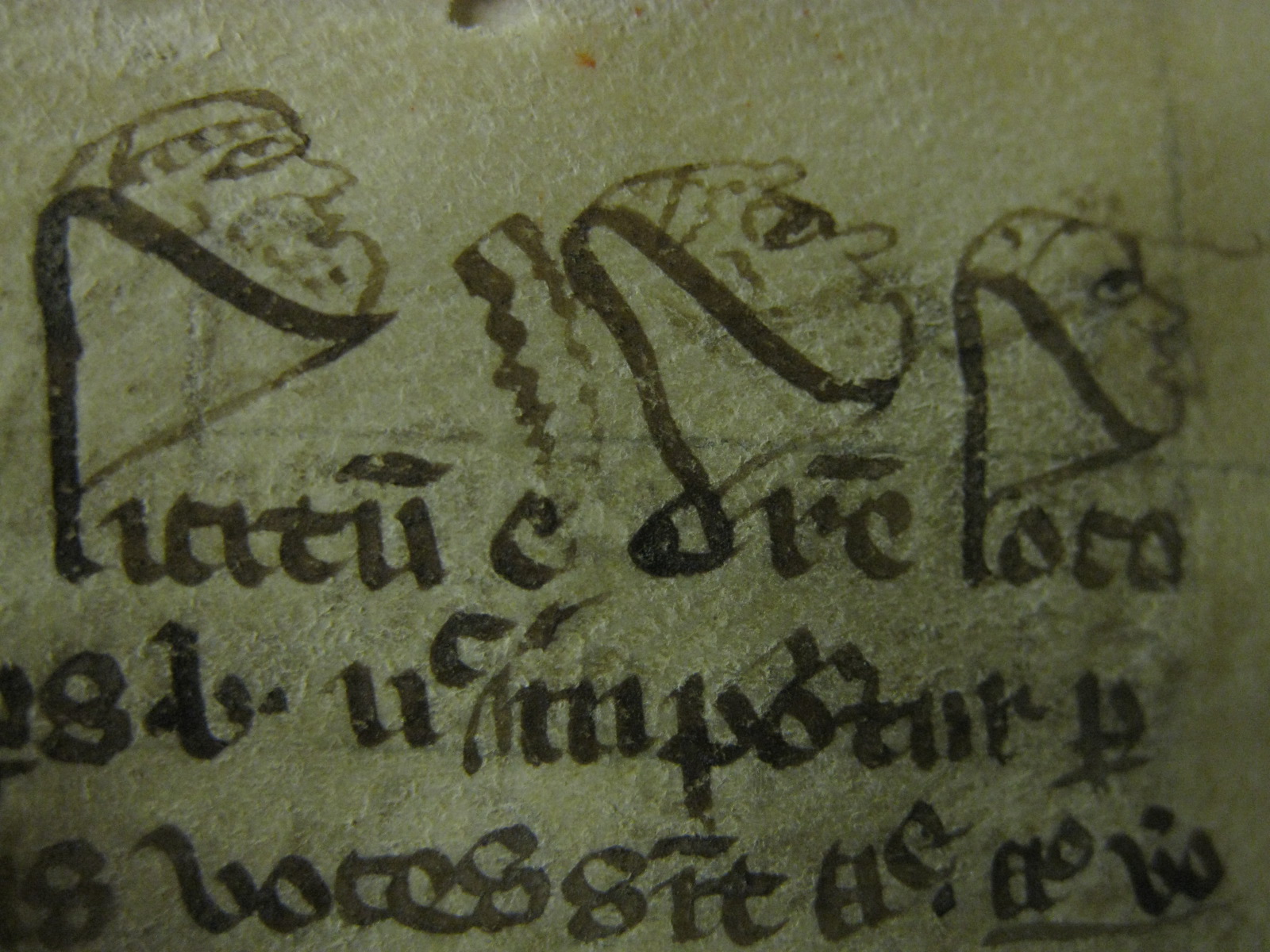 A sketch of students (or, perhaps, fellows) in a manuscript of William of Ockham's commentary on Aristotle's Physics (MS293 from the Merton College library, image courtesy of J. Walwarth). |
Michaelmas
Term
2014 (skip to HT) (skip to TT Revision Lectures) ESSENTIAL DOWNLOADS: Reading List
(notes, reading material and various other info are likely to appear here) NB:
The reading suggestions are only suggestions --- the way material is
presented in those sources is not always identical to our exposition.
See Reading List (above) for full book titles and publication info.
|
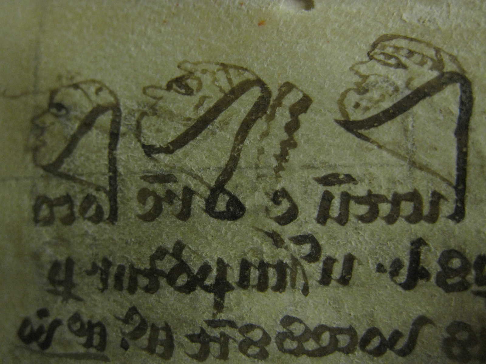 A sketch of students (or, perhaps, fellows) in a manuscript of William of Ockham's commentary on Aristotle's Physics (MS293 from the Merton College library, image courtesy of J. Walwarth). |
|
| PART I: BASIC THERMODYNAMICS |
Lectures
1-7 (Fri 31.10- Fri 14.11.14)
will be given by Professor
Andrew Boothroyd His handouts (UPDATED 2014):
Handout 1 Handout 2 Handout 3 Handout 4 Handout 5 Handout 6 Handout 7 Lecture Plan for Lectures 1-7 (UPDATED 2014) A. Boothroyd's Lecture Notes (2014) for Lectures 1-7 |
||
| You are ready to do Problem Sets 1 and 2 | |||
| PART II: KINETIC THEORY |
Lecture 1 (12:00 Wed 19.11.14)
Statistical description of a gas. Energy. Thermodynamic limit.
Lecture Notes 1
Reading: Blundell Sec 3 (a primer on probability) Kardar Chapter 2 (a more advanced primer on probability) Note:
Please make sure you have a practical command of the notions from
probability theory that I am using: random variables, their averages
(means), probability density function, joint distribution, indeoendent
random variables, change of variables for pdfs. This
may require reading a book! (for example Sinai's book suggested in the
right column) It is better to sort this out in your mind
early, otherwise initial confusion will fester and undermine you
ability to follow the rest of the course.
|
Related
mathematics: Probability and Statistics by S. Biller A superb (mathematical but accessible) course on probability theory: Ya. G. Sinai, Probability Theory: An Introductory Course An unorthodox but fascinating book on probability: E. T. Jaynes, Probability Theory: The Logic of Science (CUP 2004) A philosophical treatment of what it all means by a thinker now very much back in fashion: J. M. Keynes, A Treatise on Probability (1920, reprinted 2008) |
|
|
Lecture
2 (12:00 Thu 20.11.14)
Kinetic
calculation of pressure. Particle distribution functions. Pressure vs.
energy. Isotropic
distributions. Classical ideal gas.
Lecture
Notes 2
Reading: Blundell Sec 6.1; Pauli Sec 24; Chapman & Cowling Chapters 2, 4 (much more advanced treatment) |
|||
|
Lecture 3 (12:00 Fri 21.11.14) Maxwell's
distribution. Equation of state and temperature; heat capacity
of monatomic ideal gas. Limits of applicability of the classical ideal gas model.
Lecture
Notes 2
Reading: Blundell Sec 5 Pauli Sec 25; Chapman & Cowling Chapters 2, 4 (much more advanced treatment) |
|||
| Lecture 4 (12:00 Wed 26.11.14) Effusion. Collisions. Lecture
Notes 3
Lecture Notes 4 Reading: Blundell Sec 7 (effusion), 8 (collisions); Pauli Sec 28 (effusion), 26 (collisions); Chapman & Cowling Chapter 5 (much more advanced treatment) |
A
treatment of collisions (and derivation of Maxwell'sdistribution) from the original source: L. Boltzmann, Lectures on Gas Theory (Dover 1995) |
||
| You are ready to do Problem Set 3 | |||
|
Lecture 5 (12:00 Thu 27.11.14)
Local Maxwellian equilibrium. Conservation laws and transport equations.
|
|||
Lecture 6 (12:00 Fri 28.11.14)
Relaxation to global equilibrium. Dimensional estimates of the thermal
conductivity and viscosity. Various solutions of the transport
equations. [Diffusion.]
Reading:
Blundell
Sec 10Key thought #1: All
diffusion processes are similar (diffusion of particles, momentum,
energy...).
Key thought #2: Relaxation to equilibrium occurs in two stages: first to local equilibrium (on collision time scale, so very quickly), then to global equilibrium (diffusively, so slowly) --- both processes are collisional, but different in speed and in the nature of the physics involved. Key thought #3: Transport equations are expressions of conservation laws. We use kinetic theory to calculate the fluxes of the conserved quantities (particle number, momentum, energy). Note: Methods to solve the heat diffusion equation were covered in Mathematical Methods. There are some questions on this in Problem Set. Do go back and brush up your understanding of (i) how to find steady solutions given appropriate boundary conditions (temperature or heat flux on two boundaries), (ii) how to find time-dependent solutions given periodic boundary conditions (real frequencies, complex wavenumbers), (iii) how to find time-dependent solutions given initial conditions (real wavenumbers, complex frequencies) [see Blundell Sec 10 and Appendix C.12.]. |
Here
are some notes on dimensional analysis (from a summer school in Oxford), with an elementary treatment of a fun example of the role of viscosity: how do bubbles rise in a fluid? On diffusion, learn from the master: A. Einstein, Investigations on the Theory of the Brownian Movement (Dover 1956) [the theory of Brownian motion will be taught in the 3rd year, paper BI, but there's nothing there that you can't understand now; see also Blundell Sec 33.1] |
||
| You are ready to start working on Problem Set 4 (vacation work) | |||
| Lecture 7 (12:00 Wed 3.12.14) Kinetic
derivation of the transport equations and transport coefficients
(thermal conductivity and viscosity): the simplified "dodgy"
derivation and its critique. Kinetic expressions for fluxes and the kinetic equation. Lecture Notes 6
Reading: Blundell Sec 9 (the simplified derivation); Pauli Sec 27 (another version of this); Kardar Chapter 3 (more advanced than my treatment, includes general derivation of Boltzmann's equation and various attendant matters, in particular H theorem; treatment of fluid equations similar to mine); Kittel Sec 40, 43; Landau & Lifshitz-Kinetics Chapter 1 (hard-core Russian treatment); Chapman & Cowling Chapters 3, 6, 7, 9, 10 (hard-core Cambridge treatment) |
|||
| Lecture 8 (12:00 Thu 4.12.14) Collision operator. Local
conservation laws rederived. Solution of the kinetic equation and
calculation of fluxes. Reading:
See
Lecture 7
|
|||
| Lecture 9 (12:00 Fri 5.12.14) Solution of the kinetic equation and
calculation of fluxes. Reading:
See
Lecture 7
What I have shown you is a very
simplified version of this calculation. Do read more advanced texts and
find out how it is really done!
|
|||
 |
Hilary
Term
2015 ESSENTIAL DOWNLOADS: Reading List
LECTURES |
 |
|
| PART III: FOUNDATIONS OF STATISTICAL MECHANICS |
Lecture 1 (12:00 Wed 21.01.15)
Our programme: from microphysics to macrophysics (what we need to do to
construct the thermodynamics of a given system). Micorostates. SM
definition of pressure. Principle of maximum entropy. Lecture Notes 7
Lecture Notes 8 Reading: Binney Notes Sec 1 Schroedinger Chapter 1-2 Jaynes Sec 11.4 (assigning probabilities fairly) Blundell Sec 14.8, 15.1-15.2 (entropy, probability, information), App C.3 (Stirling's formula) My
account of the principle of maximum entropy and subsequent developments
(continued in the next lecture) owes most to J. Binney's notes,
Schroedinger's book and Jaynes' book and papers. This is not
necessarily the standard approach and I invite you to read other books
on the subject and form your own view of what makes sense. There will
be more discussion of the conceptual issues underpinning this approach
in later lectures (see Lecture Notes 12).
To avoid one particular confusion arising (which I detected in some after-lecture questions today), let me reiterate what I said in the lecture about my attitude to the equal a priori probabilities principle. The fact that it has this grand name might have suggested that it would be the foundation of what follows. In fact, I only mentioned it as a particularly simple example of a fair assignment of probabilities. In practice, we will have no use for completely isolated systems, about which we are 100% ignorant, but instead focus on systems for which at least some mean quantities can be known (measured). The statistical inferences we will make about such systems will be based on the principle of maximum entropy. This approach belongs to the Gibbs-Shannon ("canonical") family of treatments, rather than the Boltzmann one ("microcanonical"). A logic chart of both is on p. 126 of Lecture Notes 12, where I will discuss in great detail how various constructions of Statistical Mechanics compare. |
RECOMMENDED: James Binney's 2002 lecture notes on Statistical Mechanics E. T. Jaynes, Probability Theory: The Logic of Science (CUP 2004) C. Shannon's original paper: Bell System Tech. J. 27, 379 (1948) (the first in the linked issue). Also you might enjoy reading this: E. T. Jaynes, "Information Theory and Statistical Mechanics," Phys. Rev. 106, 620 (1957) On adiabatic processes (and pressure), see Binney & Skinner, Quantum Mechanics, sec 11.1-3 A very nice and readable book that has just come out: I. Ford, Statistical Physics: An Entropic Approach (Wiley 2013) although he prefers starting with the Boltzmannite microcanonical formulation, like most texts --- so I continue to recommend Schroedinger's lectures as primary reading |
|
| Lecture 2 (12:00
Thu 22.01.15) Principle of maximum entropy cont'd. Method of
Lagrange multipliers. Reading: Binney Notes Sec 3.0
Schroedinger Chapter 2-3 Blundell App C.13 (Lagrange multipliers) Note
that in order for the results derived from the maximum entropy
principle to be useful, the maximum must be quite sharp and the
resulting distributions should not have too much various (fluctuations
around the mean values should be small). All this can be quite
rigorously demonstrated for large systems and is basically related to
the quality of the "thermodynamic limit." You will find these
discussions in Schroedinger Chapters V-VI and some further relevant
maths in Jaynes Sec 11.7.
A perceptive student might wonder whether entropy is a human construct. Basically, yes, it is a measure of uncertainty that helps us make the best (unbiased) statistical inference about the state of a largely unknown system. I will discuss this issue a lot more in Lectures 6-7 (but no one stops you thinking about it until then.) |
|||
| Lecture 3 (12:00
Fri 23.01.15)
Canonical
ensemble: Gibbs distribution. Construction of thermodynamics. Additivity of entropy. Lecture
Notes 9
Reading: Binney Notes Sec 3.0.3 (composite systems) Schroedinger Chapter 2-3 Blundell Example 14.7 (Gibbs), Sec 20 (from partition function to thermodynamics) |
On
composite systems in QM, see Binney & Skinner, Quantum Mechanics, sec 6.1 If you want some intellectual stimulation of an abstract kind, see what mathematicians can do to thermodynamics: axiomatic thermodynamics by E. Lieb & J. Yngvason, Physics Reports 310, 1 (1999) (open at your own risk; you have to be over the age of consent!) An older account of Caratheodory's axiomatic thermodynamics is in Pauli Sec 11 |
||
| Lecture 4 (12:00
Wed 28.01.15) Thermal
equilibrium and the validity of the SM
definition of temperature. Heat bath and the physical interpretation of
the canonical ensemble. Mechanical and dynamical equilibria. Thermodynamic
stability, positivity of temperature
and pressure. Lecture
Notes 10
Reading: Landau & Lifshitz Sec 10 (dynamical equlibria), 12 (pressure equilbrium) Best
way to understand the stability arguments is to think about cases when
the conclusions don't apply. For example, Problem Set 5 contains some
examples of negative temperatures: why are negative tempeartures
possible there despite my arguments to the contrary in today's lecture?
|
Here's an interesting recent take on the issue of negative temperatures: J. Dunkel & S. Hilbert, Nature Phys. 10, 67 (2014) and a "popular" take on their article: I. M. Sokolov, Nature Phys. 10, 7 (2014) (note that what these people mean by "Gibbs entropy" is not the same thing as our "Gibbs-Shannon entropy") |
||
| Lecture 5 (12:00
Thu 29.01.15) SM of classical monatomic ideal gas. |
|||
| You are ready to start working on Problem Set 5 | |||
| Lecture 6 (12:00
Fri 30.01.15) Thermodynamics of ideal gas. More on
entropy: Shannon's theorem. Boltzmann entropy. Reading: Binney Notes Sec 2 (Shannon's theorem)
Shannon's paper Sec 6 and App 2 Jaynes Sec 11.3 (Shannon's theorem) We
have now encountered three sets of definitions of temperature and
pressure, viz., thermodynamical, kinetic and statistical-mechanical,
and proved they are all equivalent. Ponder how this worked and see if
you really understand the logic involved. This is a good way to
revise.
I mentioned the intriguing concept of the "thermal death of the Universe" possibly without sufficient explanation. The idea is that if the entropy of the Universe keeps increasing, we are moving towards an eventual state where it is globally maximal and so there are no gradients of any kind --- it all ends up in the ultimate boring state of deadly homogeneity --- which means, sadly for us, that no structures and so no life can survive. This realisation, the (possibly apocryphal) story goes, caused Boltzmann great distress and ultimately led to his suicide. In contrast, Schroedinger, whose understanding of statistical mechanics was (as evidenced by his book) deeper and more compelling than Boltzmann's, was quite a positive fellow, worried less about death, and indeed, among other things, wrote a book "What is Life?" which I highly recommend. He was also a Fellow of Magdalen here in Oxford until his insistence on having two wives became untenable and he moved to catholic Ireland, which, interestingly, proved more tolerant. |
If you
are interested in the history of ideas, here's a good read about Einstein's struggles with entropy, probability and the second law: A. Pais, "Subtle is the Lord..." (OUP 1982) Ch. 4 |
||
| Lecture 7 (12:00
Wed 4.02.15) Microcanonical vs.
canonical ensemble. Boltzmann vs. Gibbs. Meaning of probabilities. Second law and the loss of information. Lecture Notes 12
Reading: Schroedinger Sec 1-2 Blundell Sec 4.4-4.6 (from microcanonical to canonical) Kardar Sec 4.2, 4.6 (from microcanonical to canonical) Binney Notes Sec 5.0 Jaynes Sec 11.8 (meaning of probabilities, extra constraints etc.) Landau & Lifshitz Sec 3, 4, 7, 8 (microcanonical approach) Subjectivity of the a priori
probabilities:
if two observers have different information, will they obtain different
statistical mechanics and so different predictions? Does the heat
capacity of a box of gas depend on who is looking?! I have provided
some comments on
this in Lecture Notes 12 (pp. 130-131) --- or you can read a more
extented discussion in Jaynes Sec 11.8. There is a question in PS-5
which provides an example of what happens when a superfluous constraint
is imposed.
Lecture Notes 13There is no time this year to cover the density matrix and the way information is lost from the quantum mechanical viewpoint (which may be how it's "really" lost). You will find a treatment of this in the lecture notes and recommended readings below. Reading: Binney & Skinner Sec 6.3-6.4 Blundell Sec 15.4 Landau & Lifshitz Sec 5-6 Kardar Sec 6.5 |
Possibly the first paper that made the connection between entropy and information (and sucessfully exorcised Maxwell's demon): Leo Szilard, Z. Physik 53, 840 (1929) --- English translation in Behavioral Sci. 9, 301 (1964) Second Law: E. T. Jaynes, "Gibbs vs Boltzmann Entropies," Am. J. Phys. 33, 391 (1965) Entropy and thermodynamics from the QM perspective: E. T. Jaynes, "Information Theory and Statistical Mechanics II," Phys. Rev. 108, 171 (1957) |
||
| PART IV: STATISTICAL MECHANICS OF SIMPLE SYSTEMS |
Lectures 8-10 will be given by Professor
Andrew Boothroyd |
||
| PART V: OPEN SYSTEMS |
Lecture 11 (12:00 Thu 12.02.15) Grand
canonical
ensemble. Chemical potential. Thermodynamics of open systems. Particle
equilibrium. Lecture Notes 14
Reading: Blundell Sec 22.1-4; Kittel Sec 14; Kardar Sec 4.9; Landau & Lifshitz Sec 35-36 Note
that, like temperature, the chemical potential can be introduced purely
thermodynamically (as energy cost of adding particles to the system)
and then shown to be the same as the parameter that appears in the
grand canonical distribution. Also, instead of maximising entropy, as I
have done, one can derive the grand canonical distribution from the
microcanonical isolated-system set up by considering a small subsystem
of the world exchanging energy and particles with its surroundings.
This is how it is done in most textbooks.
|
||
| Lecture 12 (12:00 Fri 13.02.15)
Chemical potential of a classical ideal gas. Equilibria of systems in
external fields. Chemical potential and the Gibbs function. Reading: Blundell Sec 22.5-6;
Kittel Sec 14, 15; Kardar Sec 4.9; Landau & Lifshitz Sec 24, 25 |
|||
| Lecture 13 (12:00 Wed 18.02.15) Multispecies (multicomponent) systems: generalisation of the grand
canonical ensemble. Gibbs phase rule. Chemical equilibrium. Law of mass
action. Lecture Notes 15
Reading: Blundell Sec 28.5, 22.8; Kittel Sec 16; Landau & Lifshitz Sec 101-102, 104-105 Another interesting
topic that involves the use of chemical
potential but that I have not covered is the thermodynamics of
solutions. Read Landau &
Lifshitz Chapter IX if you want to find out about that (also see
Blundell & Blundell Sec 22.9 about osmotic pressure).
Disambiguation: The language at the top of p. 162 in the Lecture Notes (discussion of Gibb's phase rule) might make you think that chemical potential in phase p only depends on concentrations of that phase --- I certainly did not intend it this way, all chemical potentials in general depend on all r(m-1) unknown concentrations. |
The ionisation-recombination equilibrium (see Problem Set 6) has interesting applications to Early Universe ("the recombination epoch"). Here and here are some lecture notes (from the US) on this subject. |
||
| You are ready to do Problem Set 6 |
|||
| PART VI: QUANTUM GASES | Lecture 14 (12:00 Thu 19.02.15)
Quantum gases. Pauli exclusion principle. Partition function for
fermions and bosons. Occupation number statistics. Preview of
interesting limits. Lecture Notes 16
Reading: Blundell Chapter 29; Kardar Sec 7.1, 7.3; Landau & Lifshitz Sec 53, 54; Schroedinger Sec 8 |
||
| Lecture 15 (12:00 Fri 20.02.15) Calculations
in the continuous limit. Classical limit. Reading: Blundell Sec 30.1;
Kardar Sec 7.4; Landau & Lifshitz Sec 56; Schroedinger Sec 8 |
|||
| Lecture 16 (12:00 Wed 25.02.15) Degeneration. Degenerate
Fermi gas. Fermi
energy. Thermodynamics of Fermi gas at T=0. Finite-temperature
corrections and heat capacity. Lecture
Notes 17
Reading: Blundell Sec 30.2; Kittel Sec 19-20; Kardar Sec 7.5; Landau & Lifshitz Sec 57,58; Schroedinger Sec 8(a) |
If you
want to learn more about the thermodynamics of high-density, high-mass systems (including stability of neutron stars, which you will encounter in Problem Set 7), see Landau Chapter XI. Chandrasekhar got the 1983 Nobel Prize for his theory of the structure and evolurion of stars. Here is his Nobel lecture on the subject. |
||
| Lecture 17 (12:00 Thu 26.02.15) Degenerate
Bose gas. Bose-Einstein condensation. Lecture
Notes 18
Reading: Blundell Sec 30.3-4; Kittel Sec 21; Kardar Sec 7.6; Landau & Lifshitz Sec 62; Schroedinger Sec 8(b) |
2001 Nobel Prize ("for the achievement of Bose-Einstein condensation...") |
||
| Lectures 18-19 (on thermal
radiation) will be given by Professor
Andrew Boothroyd |
|||
| You are ready to do Problem Set 7 | |||
| PART VII: THERMODYNAMICS OF REAL GASES |
Lectures 20-24 will be given by Professor
Andrew Boothroyd His handouts:
Handout
12
Handout 13 (UPDATED 6.03.15) Handout 14 Handout 15 Additional handout: Van der Vaals Gas pVT surface of a real gas Extracurricular handout: The Third Law |
||
| You are ready to do Problem Set 8
(vacation work) |
|||
    |
Trinity
Term 2015: Revision Lectures Revision
Lecture 1 (11:00 Wed 29.04.15, Prof Boothroyd)
Revision questions Solutions to revision questions Strategy: Thermo Strategy: Stat Mech Revision Lectures 2-3 (11-12:00 Wed 20.05.15, Prof Schekochihin) I will discuss some topics from Kinetic Theory and Quantum Gases. In anticipation of the lecture, you might wish to look at the following question from past papers (all June): 2013-Q6, Q10, 2012-Q10, 2010-Q4, 2006-Q7, 2005-Q7, 2003-Q8 There will be an extended Q&A session in the 2nd hour of the lecture (12:00). Revision Lecture Notes Notes on some past questions |
    |
|
 |
|||