STATISTICAL PHYSICS
PAPER A1, SECOND YEAR
| |  |
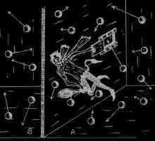
(drawing by G. Gamow) |
Alexander Schekochihin and Andrew Boothroyd
DISCLAIMER: Some of the lecture notes posted here may contain errors and imprecisions.
The notes have now been updated and the newest version is available from the 2012-13 version of the course page.
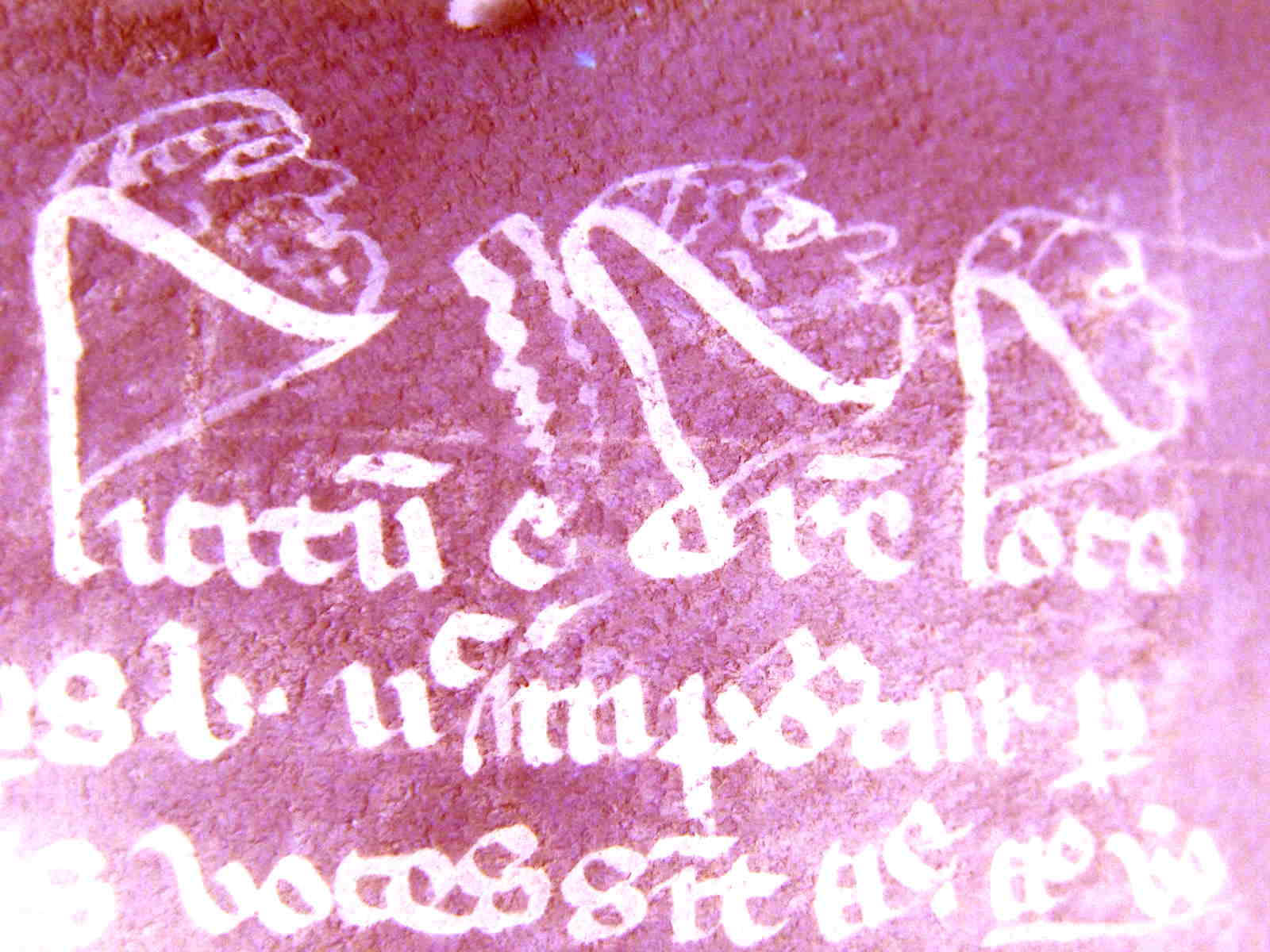
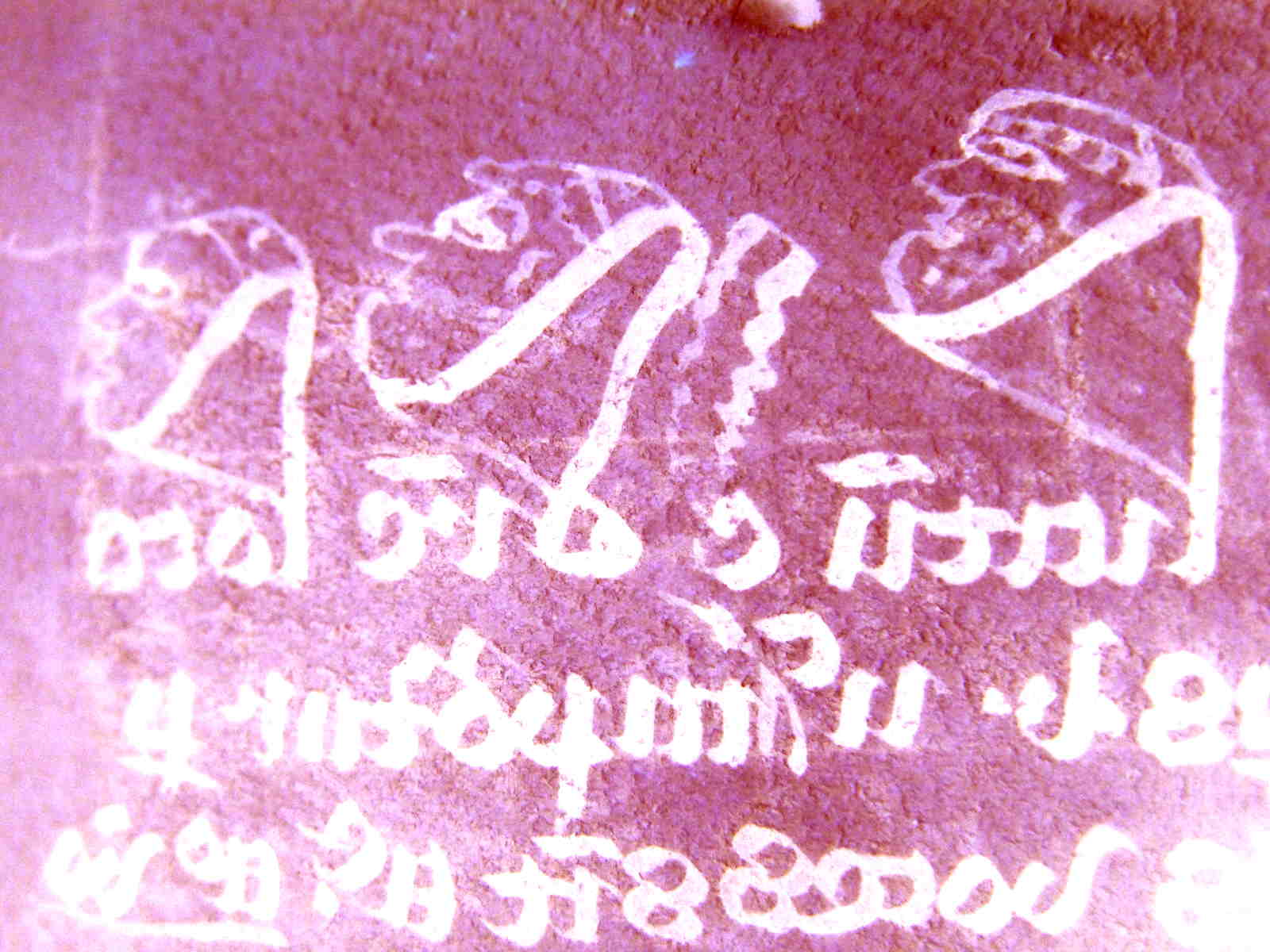
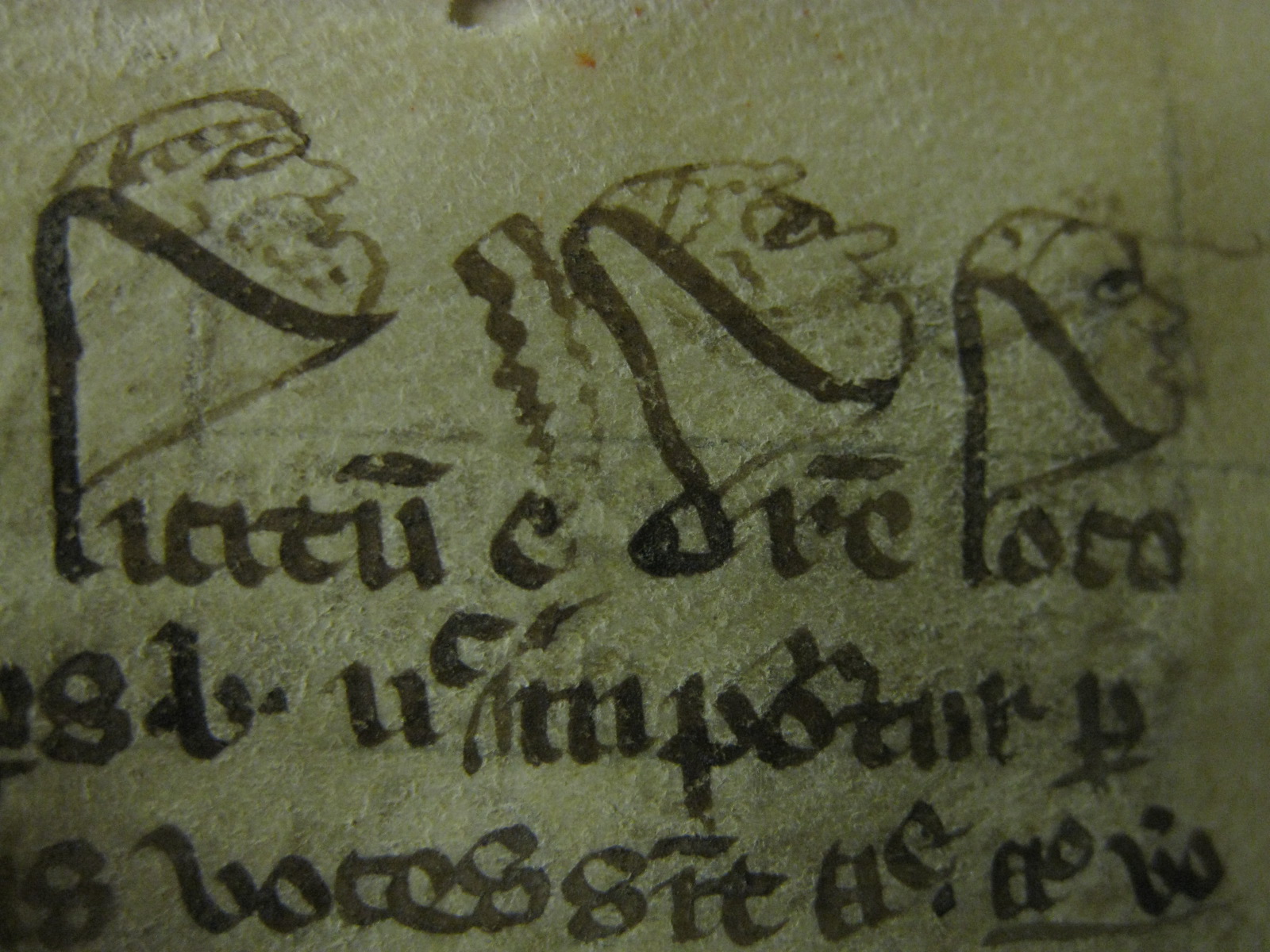 A sketch of students (or, perhaps, fellows) in a manuscript of William of Ockham's commentary on Aristotle's Physics (MS293 from the Merton College library, image courtesy of J. Walwarth). |
Michaelmas
Term
2011 (skip to HT) ESSENTIAL DOWNLOADS: Lecture Plan and Reading List (subject to changes in mid-course!) Problem Sets 1 & 2 Problem Set 3 (material to be covered in weeks 4 and 5) Problem Set 4 (from Prof Boothroyd; material to be covered in week 6) Problem Set 5 (from Prof Boothroyd; vacation work) LECTURES (notes, reading material and various other info are likely to appear here) NB:
The reading suggestions are only suggestions --- the way material is
presented in those sources is not always identical to my exposition.
See Reading List (above) for full book titles and publication info.
|
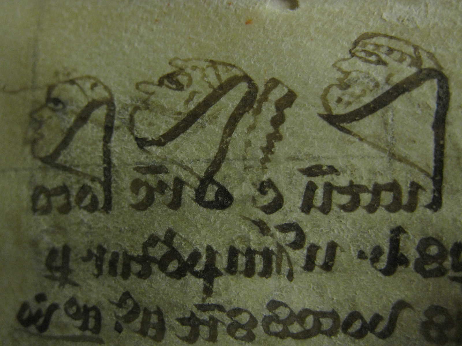 A sketch of students (or, perhaps, fellows) in a manuscript of William of Ockham's commentary on Aristotle's Physics (MS293 from the Merton College library, image courtesy of J. Walwarth). |
|
| PART I: KINETIC THEORY | Lecture 1 (12.10.11)
Statistical description of a gas. Particle distribution function.
Calculation of pressure in terms of particle distribution. Isotropic
distributions. Summary Sheet I;
Lecture Notes 1 Reading: Blundell Sec 3, 6.1; Pauli-Thermo Sec 24 (pressure); Kardar Chapter 2 (a more advanced primer on probability); Chapman & Cowling Chapter 2 Note:
Please make sure you have a practical command of the notions from
probability theory that I have introduced (pdfs, averages, joint
distributions, independent variables, change of variables etc.). This
may require reading a book! It is better to sort this out in your mind
early, otherwise initial confusion will fester and undermine you
ability to follow the rest of the course.
|
Related mathematics: Probability and Statistics by S. Biller A good (mathematical but accessible) course on probability theory: Ya. G. Sinai, Probability Theory: An Introductory Course |
|
| Lecture 2 (13.10.11) Isotropic
distributions (cont'd). Classical ideal gas. Maxwell’s distribution. Temperature, pressure,
equation of state for a classical ideal gas. Effusion. Summary Sheet II;
Lecture Notes 2 Reading: Blundell Sec 5, 6.2, 7; Pauli-Thermo Sec 25, 28; Chapman & Cowling Chapter 4 (much more advanced treatment) Note: The definition of
v_th is completely arbitrary and is a matter of covenvience (easy to
remember the Maxwellian in this form). This definition can vary from
book to book (with factors of 2 creeping up if, e.g., you define
<v_x^2>=v_th^2). The definition of temperature on the other hand,
is stable across literature: kT/2 = m<v_x^2>/2 (mean energy per
degree of freedom).
|
|||
| Lecture 3 (19.10.11) Collisions: cross-section, collision rate, mean free path. Qualitative treatment of collisional transport: diffusion. Lecture Notes 3
Reading: Blundell Sec 8 (collisions), App C.12 (solution of diffusion equation); Pauli-Thermo Sec 26; Chapman & Cowling Chapter 5 (much more advanced treatment); Pauli-Stat Mech Sec 18 (diffusion) Note: I showed in the
lecture that amplitudes of the ihomogeneities diffuse away as ~
exp(-Dk^2 t). This highlights the very fundamental property of
diffusive processes: diffusion time t ~ L^2/D, where L is the typical
scale of inhomogeneity. Generally the distance travelled by diffusing
("random walking") particles is L~sqrt(t), while for unimpeded
("ballistic") motion, L ~ t. Diffusion is slower because particles are
randomly deflected by collisions and the distance traveled accumulates
only on average.
|
|||
| Lecture 4 (20.10.11) Qualitative
treatment of collisional transport (cont'd): fluxes, viscosity, heat
conductivity, notion of steady state solutions to diffusion equations. Summary Sheet III (coming soon);
Lecture Notes 4 Reading: Blundell Sec 9, 10; Pauli-Thermo Sec 27; Chapman & Cowling Chapter 6 Note how different
calculations of the transport coefficients
(in my lectures or in the reading material above) give different
numerical prefactors. All of this is in fact qualitative. In Lectures
5-6, you will get a taste of how a quantitatively correct calculation
is constructed.
|
Related mathematics: Mathematical Methods by J. Magorrian (where you will learn how to solve the heat diffusion equation) |
||
| Lecture 5 (26.10.11) [non-examinable] Kinetic equation with simplified (BGK) collision operator. Derivation of fluid equations. Lecture 6 (27.10.11) [non-examinable] Derivation of fluid equations (cont'd). Calculation of collisional transport terms: heat flux and viscous stress. Lecture Notes 5
Reading: Kardar Chapter 3 (more advanced than my treatment, includes general derivation of Boltzmann's equation and various attendant matters, in particular H theorem; treatment of fluid equations similar to mine); Landau & Lifshitz-Kinetics Chapter 1 (hard-core Russian treatment); Chapman & Cowling Chapters 3, 7, 9, 10 (hard-core Cambridge treatment); Pauli-StatMech Chapter 1 (a version of the above) Note that the result of
my calculation of viscous stress was a much more general expression
than in Lecture 4: velocities and gradients were allowed to be in any
direction. Convince yourself that if you assume velocity is in the x
direction only and its gradient in the z direction, you recover the old
result!
|
|||
|
PART II: FOUNDATIONS OF STATISTICAL MECHANICS |
Lecture 7 (28.10.11) Microstates. Equal a priori probabilities. Principle of maximum entropy. Lecture 8 (2.11.11) Shannon entropy [non-examinable]. Method of Lagrange multipliers. Equal probabilities in a closed system. Canonical ensemble and the Gibbs distribution. Lecture Notes 6
Reading: Binney Sec 2, 3.0; Schroedinger Sec 1-2; Blundell Sec 14.8, 15 (entropy, info theory; note examples 14.6, 14.7!), App C.3 (Stirling's formula), C.13 (Lagrange multipliers) Note that there are
several different possible logical progressions for introducing Statistical Mechanics and Thermodynamics. All of these different
schemes are represented in the books on your reading list.
--- The way it is done in my lectures owes most to J. Binney's notes. It is also, mostly, the same philosophy as adopted in the little book by Schroedinger, although, formally speaking, he introduces entropy post hoc rather than as the fundamental measure of uncertainty to be optimised (his book is not easy, but I recommend reading it, or at least its first two sections, strongly to you as an example of a physicist writing not only cogently and lucidly, but also beautifully). This approach essentially originated with J. W. Gibbs, as opposed to the more traditional viewpoints mentioned below and going back to Boltzmann and Maxwell (although Maxwell apparently was one of the few physicists at the time to appreciate what Gibbs did). --- In Blundell, definition of temperature and the canonical ensemble come first (Sec 4), then all of thermodynamics is developed (Sec 11-14.7, 16-18), and finally probabilistic/informational approach to entropy (Sec 14.8-15) is a postscript; thermodynamics is later rederived from the partition function (Sec 20). If you read Sec 4 and 20 after my Lecture 10, you'll be able to see how this approach gets to the same results as I did. Prof Boothroyd will derive most of the standard practical thermodynamics material in the second half of this term's course. --- In many other theoretically advanced books (Landau & Lifshitz, Pauli, Kardar), the starting point is the equal a priori probabilities postulate and the microcanonical distribution (in fact, implicitly, that is the case in Blundell as well; see Sec 14.5). If I have time to cover this topic towards the end of my lectures, you can read the relevant chapters in those books and decide which approach you like better. It is because these books employ different logical schemes that the chapters from them recommended in my reading suggestions appear in non-sequential order. A summary table of the two approaches is on the last page of Lectures Notes 11. As far as your syllabus is concerned, you are mostly examinable on the main practical results, which are the same for all these treatments, but not on the underlying theoretical framework. It is unlikely, however, that you will have a true appreciation of those results unless you manage to make sense of one of the logical schemes for getting them. My view is of course that the way I am presenting the subject is the clearest, but you are welcome to take this critically and decide whether the Boltzmannites or the Gibbsians have your allegiance. |
RECOMMENDED: James Binney's 2002 lecture notes on Statistical Mechanics You could also look at these (a different exposition): R. Fitzpatrick's lecture notes (from UT Austin) C. Shannon's original paper: Bell System Tech. J. 27, 379 (1948) (the first in the linked issue). Possibly the first paper that made the connection between entropy and information (and sucessfully exorcised Maxwell's demon): Leo Szilard, Z. Physik 53, 840 (1929) --- English translation in Behavioral Sci. 9, 301 (1964) An interesting set of reads on entropy, information theory etc.: books and articles by E. T. Jaynes |
|
| Lecture 9 (3.11.11)
Energy and entropy, their additivity. Adiabatic processes. Definition
of pressure (and other response functions to external parameters).
Fundamental equation of thermodynamics. Functions of state. Lecture Notes 7
Reading: Binney Sec 1, 3.0; Schroedinger Sec 2; Landau & Lifshitz-Stat Phys Sec 11 (ad. process), 12 (pressure); Blundell Sec 11.1 (functions of state) |
|||
| Lecture 10 (4.11.11) Zeroth
law. Meaning of temperature. Thermal and mechanical equilibrium. First
law. Heat and work. Reversibility. Second law. Lecture Notes 8
Reading: Binney Sec 3.0; Schroedinger Sec 2; Kardar Sec 1.2 (zeroth law, empirical temperature), 1.3 (first law); Pauli-Thermo Sec 2 (temperature), 3-4, 6 (first law), 12 (free energy, heat capacity); Landau & Lifshitz-Stat Phys Sec 9 (temperature), 10 (stability), 12 (mech. equilibrium), 13 (work and heat), 15 (free energy); Blundell Sec 4 (temperature, canonical ensemble etc. by a different route), 11.2 (first law), 11.3 (heat capacity), 14.3 (fund. eqn of thermo. from first law), 20 (partition function and calculation of functions of state from it) Note:
At the end of the lecture, I referred to the intriguing concept of
"thermal death of the Universe" possibly without sufficient
explanation. The idea is that if the entropy of the Universe keeps
increasing, we are moving towards an eventual state where it is
globally maximal and so there are no gradients of any kind --- it all
ends up in the ultimate boring state of deadly homogeneity --- which
means, sadly for us, that no structures and so no life can survive.
This realisation, the (possibly apocryphal) story goes, caused
Boltzmann great distress and ultimately led to his suicide. In
contrast, Schroedinger, whose understanding of statistical mechanics
was (as evidenced by his book) possibly deeper and more compelling than
Boltzmann's, was quite a positive fellow, worried less about death, and
indeed, among other things, wrote a book "What is Life?" which I highly
recommend. He was also a Fellow of Magdalen here in Oxford until his
insistence on having two wives became untenable and he moved to
catholic Ireland, which, interestingly, proved more tolerant.
|
What mathematicians can do to thermodynamics: axiomatic thermodynamics by E. Lieb & J. Yngvason, Physics Reports 310, 1 (1999) (open at your own risk; you have to be over 18!) An older account of Caratheodory's axiomatic thermodynamics is in Pauli-Thermo Sec 11 |
||
| Lecture 11 (9.11.11) How and what to
calculate: free energy, equation of state, heat capacity. Statistical
mechanics of classical ideal gas. Density of states.
Distinguishability, extensivity of entropy and Gibbs paradox. Summary Sheets IV & V (coming soon);
Lecture Notes 9 Lecture Notes 10 Reading: Blundell Sec 21.1-5; Kardar Sec 4.4-4.5; Schroedinger Sec 4a, 8 (the beginning of it) |
|||
| Lecture 12 (10.11.11) Statistical
mechanics of classical ideal gas (cont'd). Neglect of quantum correlations. N-particle partition function.
Entropy, energy, equation of state and heat capacity for monatomic
ideal gas. Equivalance of the kinetic and stat-mech definitions of
temperature and pressure. [non-examinable:] Microcanonical ensemble. Construction of
thermodynamics from it. Relationship to canonical ensemble. Lecture Notes 11
(summary of both approaches is on the last page of these notes) Reading: Kardar Sec 4.2 (microcanonical and consequences), 4.6 (canonical from micro); Blundell Sec 4.4, 4.6 (canonical from micro); Landau & Lifshitz Sec 3, 4, 7, 8; Pauli-Stat Mech Sec 8, 9, 10; Binney Sec 5.0 (micro from canonical) |
|||
|
PART III: BASIC THERMODYNAMICS |
Lectures 13-22 will be delivered by Professor Andrew Boothroyd |
||
|
PART IV: STATISTICAL MECHANICS AND THERMODYNAMICS OF SIMPLE SYSTEMS |
Handout 6 Handout 7 Handout 8 |
||
 |
Hilary Term
2012 ESSENTIAL DOWNLOADS: Problem Set 6 (material covered in weeks 1 and 2) Problem Set 7 (material covered in weeks 2 and 3) Problem Set 8 (from Prof Boothroyd, material covered in weeks 4 and 5) LECTURES |
 |
|
| PART V: FURTHER STATISTICAL MECHANICS: OPEN SYSTEMS AND QUANTUM GASES |
Lecture 1 (18.01.12) Ensembles redux. Grand canonical ensemble. Chemical potential. Thermodynamics of open systems. Lecture 2 (19.01.12) Particle equilibrium. Chemical potential and the Gibbs function. Chemical potential of classical ideal gas. Generalisation of grand canonical approach to multispecies (multicomponent) systems.
Lecture Notes 12
Reading: Blundell Sec 22.1-5; Kittel Sec 14; Kardar Sec 1.7-1.8, 4.9; Landau & Lifshitz Sec 24, 25, 35-36; Pauli-Stat Mech Sec 14(a) Note
that, like temperature, the chemical potential can be introduced purely
thermodynamically (as energy cost of adding particles to the system)
and then shown to be the same as the parameter that appears in the
grand canonical distribution. Also, instead of maximising entropy, as I
have done, one can derive the grand canonical distribution from the
microcanonical isolated-system set up by considering a small subsystem
of the world exchanging energy and particles with its surroundings.
This is how it is done in most textbooks.
|
RECOMMENDED (in addition to the Reading List): C. Kittel, Elementary Statistical Physics |
|
| Lecture 3 (20.01.12) Multispecies systems continued. Chemical equilibrium. Summary Sheet VI
Lecture Notes 13 Reading: Blundell Sec 22.6-8; Kittel Sec 16; Landau & Lifshitz Sec 101-102, 104-105; Pauli-Stat Mech Sec 14(b) There
is another interesting topic that involves the use of chemical
potential but that I have not covered: solutions. Read Landau &
Lifshitz Chapter IX if you want to find out about that (also see
Blundell & Blundell Sec 22.9 about osmotic pressure).
|
The ionisation-recombination equilibrium (see Problem Set 6) has interesting applications to Early Universe ("the recombination epoch"). Here and here are some lecture notes (from the US) on this subject. |
||
| Lecture 4 (25.01.12)
Quantum gases. Pauli exclusion principle. Partition function for
fermions and bosons. Occupation number statistics. Preview of
interesting limits. Reading: Blundell Chapter 29;
Kardar Sec 7.1, 7.3; Landau & Lifshitz Sec 53, 54; Schroedinger Sec 8; Pauli-Stat Mech Sec 24 I mentioned in passing
that the expression for the entropy of a quantum ideal gas in terms of
mean occupation numbers (Lecture Notes-14, p.122) is valid also out of
equilibrium and one can obtain Fermi-Direc and Bose-Einstein statistics
by maximising this entropy subject to fixed mean energy and particle
number. This is discussed in more detail in Landau Sec 55 and 40.
Lecture 5 (26.01.12) Quantum gases continued. Calculations in the continuous limit. Classical limit. Degeneration. Lecture Notes 14
Reading: Blundell Sec 30.1; Kardar Sec 7.4; Landau & Lifshitz Sec 56; Schroedinger Sec 8; Pauli-Stat Mech Sec 24(a,b1) Here's a slightly
disturbing calculation one can do. Why do we treat the (average) number
of particles as given? After all, mass is energy, so we could
completely relax this constraint and instead include mc^2 into the
single-particle energy levels in the grand paratition function.
Mathematically, this amount to replacing mu in all our results by -mc^2
(energy cost of a particle). Then eq. (1) in the notes is no longer an
equation for mu but rather determines the density of matter, n=N/V.
Assume room temperature, use mc^2>>>>>kT, and hence
calculate n. It comes out so tiny that one must wonder why there is any
matter at all left in the world. Why do you think?
|
|||
| Lecture 6 (27.01.12) Degenerate Fermi gas. Lecture Notes 15
Reading: Blundell Sec 30.2; Kittel Sec 19-20; Kardar Sec 7.5; Landau & Lifshitz Sec 57,58; Schroedinger Sec 8(a); Pauli-Stat Mech Sec 24(b2) To gain proper mastery
and understanding of the calculations of the last three lectures, I
urge you to work through them and fill in the blanks (also, reworking
everything in the ultrarelativistic limit would be a good exercise --- you are forced to do it in Problem Set 7).
There's only so much one can grasp by passively taking it all in in
lectures, which must needs proceed apace, but you now have heard enough
to be able to start doing some serious calculations on your own!
Speaking of which, if you find the homeworks too easy, both Landau's
and Kardar's books have more challenging reads and exercises to offer
(some of them with solutions). I also renew my recommendation of
Schroedinger's little book as a particularly fun read.
Let me reiterate a point I made very quickly at the end of the lecture. Heat capacity of degenerate electrons in metals will be ~T. The other contribution to the heat capacity of a metal will come from the lattice --- recall Einstein's model of a solid introduced in MT. However, at low temperatures, that goes as ~T^3. Thus, at low temperatures, electrons will dominate. At what temperature will the lattice contribution become important? |
If you want to learn more about the thermodynamics of high-density, high-mass systems (including stability of neutron stars, which you encountered in Problem Set 6), see Landau Chapter XI. Chandrasekhar got the 1983 Nobel Prize for his theory of the structure and evolurion of stars. Here is his Nobel lecture on the subject. |
||
| Lecture 7 (1.02.12) Degenerate Bose gas and Bose-Einstein condensation. Summary Sheet VII
Lecture Notes 16 Reading: Blundell Sec 30.3-4; Kittel Sec 21; Kardar Sec 7.6; Landau & Lifshitz Sec 62; Schroedinger Sec 8(b); Pauli-Stat Mech Sec 24(b3) Looking
forward, I hope you realise that in Q1 of Problem Set 7 you worked out
the entire theory of photon gas (mu=0, - sign in the denominators) and
electron-positron pair gas (mu=0, + sign in the denominators). Note
also the basic similarity between the non-condensed part of a Bose gas
at T<T_c and photon gas. The difference is that the former is
non-relativistic.
|
2001 Nobel Prize ("for the achievement of Bose-Einstein condensation...") |
||
| Lectures 8-14 will be delivered by Professor Andrew Boothroyd |
|||
| PART VI: FURTHER THERMODYNAMICS: REAL GASES AND PHASE TRANSITIONS |
Handout 10 Handout 11 Handout 12 Handout 13 |
||
 |